書籍「ベイズ信号処理(関原 謙介)」の「第10章 数値実験」の計算例をPythonで実行しました.問題設定やアルゴリズムについては書籍を参照してください.

出版社のページで正誤表やMATLABコードが公開されています.MATLABコードをそのままPythonにしてもうまくいかず,試行錯誤が必要でした.
ベイズ信号処理 - 共立出版
使っているライブラリ・関数は以下を参照してください.
データ生成
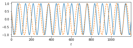
# パラメータ
SNR = 1
d = 300

## センサー位置 (x座標)
xmin, xmax = -1000, 2000
pos_sensor = np.arange(xmin, xmax+1, 10)

tmin, tmax = 0, 1200-1
t = np.arange(tmin, tmax+1, 1)

# 信号
s1 = np.cos(2*np.pi*t/77 + np.pi/3.3).reshape(1, -1)
s2 = np.cos(2*np.pi*t/97 + np.pi/3.3).reshape(1, -1)

def f(X, x0, d):
    return 1/((X-x0)**2+d**2)

sig1 = f(pos_sensor, 300, d).reshape(-1, 1) @ s1
sig2 = f(pos_sensor, 700, d).reshape(-1, 1) @ s2
sig = sig1 + sig2

# ノイズ
Noise = np.random.normal(loc=0.0, scale=1, size=sig.shape)
Noise *= np.linalg.norm(sig, 'fro')/np.linalg.norm(Noise, 'fro')  # SNR=1
Noise *= 1/SNR
y = sig + Noise

# データのプロット
num = 1
fig = plt.figure(figsize = (6.4, 4.8 * num / 2), tight_layout = True)
axes = [fig.add_subplot(num, 1, i + 1) for i in range(num)]
axes[0].plot(t, s1.flatten())
axes[0].plot(t, s2.flatten(), '--')
for ax in axes:
    ax.set_xlim(tmin, tmax)
    ax.set_xlabel('$t$')
plt.show()
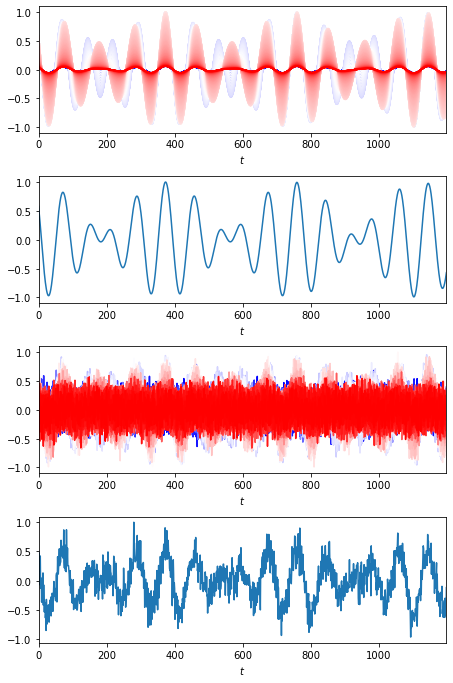
# 表示するセンサー番号
channel = 150

num = 4
fig = plt.figure(figsize = (6.4, 4.8 * num / 2), tight_layout = True)
axes = [fig.add_subplot(num, 1, i + 1) for i in range(num)]
for i in range(sig.shape[0]):
    axes[0].plot(t, sig[i,:]/np.max(sig), c=cm.bwr(i/sig.shape[0]))
axes[1].plot(t, sig[channel-1,:]/np.max(sig[channel-1,:]))
for i in range(sig.shape[0]):
    axes[2].plot(t, y[i,:]/np.max(y), c=cm.bwr(i/sig.shape[0]))
axes[3].plot(t, y[channel-1,:]/np.max(y[channel-1,:]))
for ax in axes:
    ax.set_xlim(tmin, tmax)
    ax.set_xlabel('$t$')
plt.show()
EMアルゴリズムを使う方法
因子数$L$を固定値として与える.def BayesFactorAnalysis(nloop, y, L): """ Parameters: y: (M, K), M:x座標の点数, K:時間点数 L: 因子数 Returns: A: (M, L), 混合行列 Lambda: (M, M), ノイズの精度行列 A @ ubar: (M, K), 信号成分(ノイズを除去したデータ) ubar: (L, K), 因子活動 """ # init M, K = y.shape ## AをデータのSVDで初期化 U, S, _ = np.linalg.svd(y, full_matrices=False) A = U[:, :L] @ np.diag(S[:L]) ## ノイズの精度行列をデータの分散の対角成分で初期化 Ryy = y @ y.T Lambda = K * np.diag(1/np.diag(Ryy)) # EMアルゴリズム for _ in range(nloop): ## E step: (6.10), (6.11) Gamma = (A.T @ Lambda @ A) + np.identity(L) invGamma = inv_cholesky(Gamma) ubar = np.linalg.solve(Gamma, A.T @ Lambda @ y) ## (6.15), (6.16), (6.17) Ruu = (ubar @ ubar.T) + (K * invGamma) Ruy = ubar @ y.T Ryu = Ruy.T ## M step: (6.18), (6.23) A = Ryu @ inv_cholesky(Ruu) Lambda = K * np.diag(1/np.diag(Ryy - (A @ Ruy))) return A, Lambda, Ryu @ np.linalg.solve(Ruu, ubar), ubar
VB(変分ベイズ)EMアルゴリズムを使う方法
因子数$L$を大きめに与え,$L$を推定させる.def VariationalBayesFactorAnalysis(nloop, y, L): """ Parameters: y: (M, K), M:x座標の点数, K:時間点数 L: 因子数 Returns: A: (M, L), 混合行列 Lambda: (M, M), ノイズの精度行列 A @ ubar: (M, K), 信号成分(ノイズを除去したデータ) ubar: (L, K), 因子活動 """ # init M, K = y.shape ## AをデータのSVDで初期化 U, S, _ = np.linalg.svd(y, full_matrices=False) A = U[:, :L] @ np.diag(S[:L]) ## ノイズの精度行列をデータの分散の対角成分で初期化 Ryy = y @ y.T Lambda = K * np.diag(1/np.diag(Ryy)) ## invPsi = np.identity(L) alpha = np.diag(1/np.diag((A.T @ Lambda @ A)/M + invPsi)) # EMアルゴリズム for _ in range(nloop): ## E step: (8.21), (8.22) Gamma = (A.T @ Lambda @ A) + np.identity(L) + (M * invPsi) invGamma = inv_cholesky(Gamma) ubar = np.linalg.solve(Gamma, A.T @ Lambda @ y) ## (6.15), (6.16), (6.17) Ruu = (ubar @ ubar.T) + (K * invGamma) Ruy = ubar @ y.T Ryu = Ruy.T ## M step: (8.33), (8.31) Psi = Ruu + alpha invPsi = inv_cholesky(Psi) A = Ryu @ invPsi ## (8.47) Lambda = K * np.diag(1/np.diag(Ryy - (A @ Ruy))) ## (8.40) alpha = np.diag(1/np.diag((A.T @ Lambda @ A)/M + invPsi)) return A, Lambda, Ryu @ np.linalg.solve(Psi, ubar), ubar
実行結果
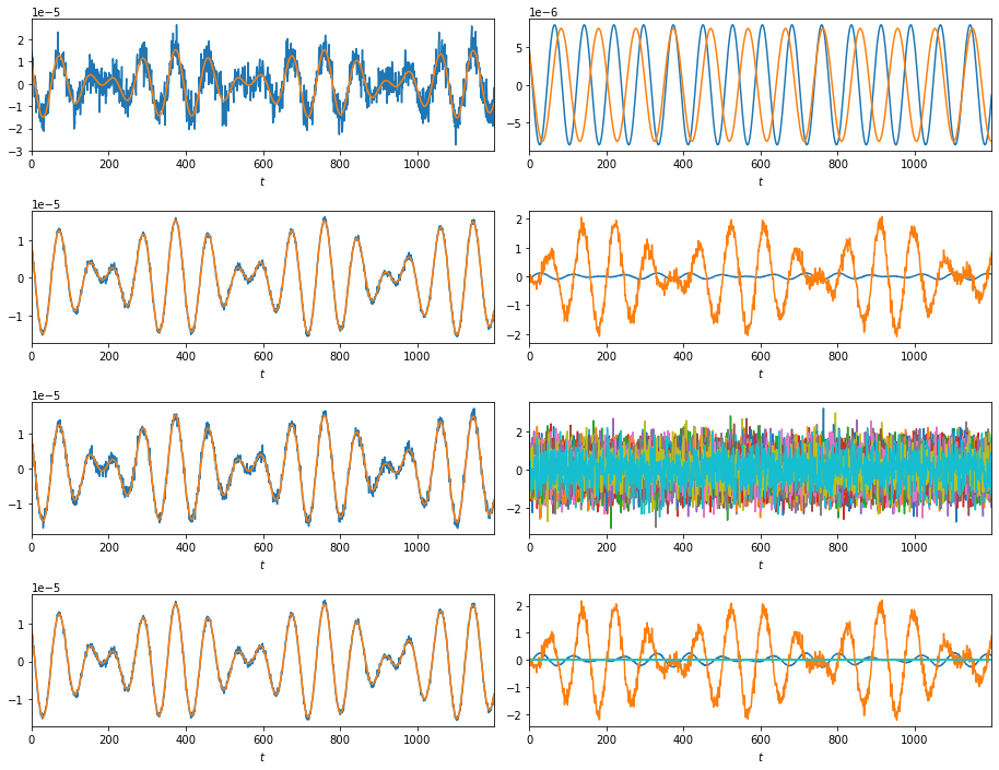
_, _, BFA_Au2, BFA_u2 = BayesFactorAnalysis(nloop=200, y=y, L=2)
_, _, BFA_Au30, BFA_u30 = BayesFactorAnalysis(nloop=200, y=y, L=30)
_, _, VBFA_Au30, VBFA_u30 = VariationalBayesFactorAnalysis(nloop=400, y=y, L=30)


num = 4*2
fig = plt.figure(figsize = (6.4*2, 4.8 * num / 2), tight_layout = True)
axes = [fig.add_subplot(num, 2, i + 1) for i in range(num)]
axes[0].plot(t, y[channel-1,:])
axes[0].plot(t, sig[channel-1,:])
axes[1].plot(t, sig1[channel-1,:].T)
axes[1].plot(t, sig2[channel-1,:].T)
axes[2].plot(t, BFA_Au2[channel-1,:])
axes[2].plot(t, sig[channel-1,:])
axes[3].plot(t, BFA_u2.T)
axes[4].plot(t, BFA_Au30[channel-1,:])
axes[4].plot(t, sig[channel-1,:])
axes[5].plot(t, BFA_u30.T)
axes[6].plot(t, VBFA_Au30[channel-1,:])
axes[6].plot(t, sig[channel-1,:])
axes[7].plot(t, VBFA_u30.T)
for ax in axes:
    ax.set_xlim(tmin, tmax)
    ax.set_xlabel('$t$')
plt.show()
一番上は(ノイズを加えた)もとの信号.
左の列にはノイズ除去後の信号と,もとの(ノイズなしの)信号をプロットした.
右列には因子をプロットした.