Pythonで拡張カルマンフィルタ

以下の書籍の例をPythonで試しました．
また，拡張カルマンフィルタを使うと，（当然）線形カルマンフィルタの例も計算できることを確かめます．

作者:足立修一,丸田一郎
東京電機大学出版局

拡張カルマンフィルタ

拡張カルマンフィルタ

非線形関数$\bm{f}, h$を使ったモデルによって記述される，以下のスカラ時系列$\{y(k)\}$を考える．

\begin{aligned}
\begin{cases}
\, \bm{x}(k + 1) = \bm{f} \bigl(\bm{x}(k)\bigr) + \bm{b} v(k)
& (\text{状態方程式}) \\
\, y(k) = h \bigl(\bm{x}(k)\bigr) + w(k)
& (\text{観測方程式})
\end{cases}
\end{aligned}

拡張カルマンフィルタ（Extended Kalman filter - Wikipedia，EKF）では，非線形関数を線形近似して，線形カルマンフィルタに帰着させる．

以下も参考になるかも：
非線形カルマンフィルタの基礎

numpyによる実装

事後状態推定値$\hat{x}$，事後誤差共分散行列$P$，カルマンゲイン$\bm{g}$を返す関数：

def ekf(f, h, dfdx, B, dhdx, Q, R, y, xhat, P):
    """
    x(k+1) = f(x(k)) + Bv(k)
    y(k) = h(x(k)) + w(k)
    """
    xhatm = f(xhat)
    A = dfdx(xhat)
    Pm = (A @ P @ A.T) + Q * (B @ B.T)
    CT = dhdx(xhatm)
    C = CT.T
    G = (Pm @ C) / ((CT @ Pm @ C) + R)
    xhat_new = xhatm + G * (y - h(xhatm))
    P_new = (np.eye(len(A)) - (G @ CT)) @ Pm
    return xhat_new, P_new, G

上の関数を繰り返し適用して，$\hat{x}, \bm{g}$をすべての時系列で計算する関数：

def calc_timeseries_ekf(N, f, h, dfdx, B, dhdx, Q, R, y, x0, P_ekf):
    xhat_ekf = [x0]
    G0 = np.empty(x0.shape)
    G0[:] = np.nan
    G_ekf = [G0]
    for k in range(1, N):
        xhat_new, P_new, G = ekf(f, h, dfdx, B, dhdx, Q, R, y[k], xhat_ekf[-1], P_ekf)
        xhat_ekf.append(xhat_new)
        G_ekf.append(G)
        P_ekf = P_new
    xhat_ekf = np.array(xhat_ekf)
    G_ekf= np.array(G_ekf)
    return xhat_ekf, G_ekf

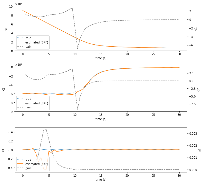
物体の落下運動

書籍7.4の例を，上の関数でシミュレーションする．
背景については，次が参考になるかも．
Unscented Kalman Filterを用いた力学系の状態およびパラメータ推定
http://lab.cntl.kyutech.ac.jp/~nishida/lecture/psc/no9.pdf

次の記事で，Unscented Kalman Filter (UKF)との比較をしています．
PythonでUnscented Kalman Filter (UKF) - Notes_JP

import numpy as np
import matplotlib.pyplot as plt
import matplotlib.ticker as ptick

# --- パラメータ ---
rho = 1.23
g = 9.81
eta = 6e3
M = 3e4
a = 3e4

T = 0.5
EndTime = 30
N = int(EndTime / T + 1)
time = T * np.arange(0, N)
n = 3
R = 4e3
Q = 0
B = np.array([
    [0],
    [0],
    [0]
])

# --- 関数 ---
def f(x):
    x1, x2, x3 = x
    x1, x2, x3 = x1.item(0), x2.item(0), x3.item(0)
    res = np.array([
        [x1 + T * x2],
        [x2 + T * (0.5 * rho * np.exp(- x1 / eta) * (x2 ** 2) * x3 - g)],
        [x3]
    ])
    return res

def h(x):
    x1, x2, x3 = x
    x1, x2, x3 = x1.item(0), x2.item(0), x3.item(0)
    return np.sqrt((M ** 2) + ((x1 - a) ** 2))

def dfdx(x):
    x1, x2, x3 = x
    x1, x2, x3 = x1.item(0), x2.item(0), x3.item(0)
    res = np.array([
        [1, T, 0],
        [- T * 0.5 * (rho / eta) * np.exp(- x1 / eta) * (x2 ** 2) * x3,
         1 + T * rho * np.exp(- x1 / eta) * x2 * x3,
         T * 0.5 * rho * np.exp(- x1 / eta) * (x2 ** 2)
        ],
        [0, 0, 1]
    ])
    return res

def dhdx(x):
    x1, x2, x3 = x
    x1, x2, x3 = x1.item(0), x2.item(0), x3.item(0)
    res = np.array([
        [(x1 - a) / h(x), 0, 0]
    ])
    return res

# --- 真値，　測定値 ---
w = np.random.normal(loc = 0.0, scale = np.sqrt(R), size = N)
x = [np.array([
    [9e4], 
    [-6e3],
    [3e-3]
])]
y = [h(x[-1]) + w[0]]

for k in range(N - 1):
    x.append(f(x[-1]))
    y.append(h(x[-1]) + w[k + 1]) 
x = np.array(x)

# --- EKF ---
P_ekf = np.array([
    [9e3, 0, 0],
    [0, 4e5, 0],
    [0, 0, 0.4]
])

xhat_ekf, G_ekf = calc_timeseries_ekf(N, f, h, dfdx, B, dhdx, Q, R, y, x[0], P_ekf)

# --- プロット ---
fig_num = 3
fig = plt.figure(figsize = (10, 3 * fig_num), tight_layout = True)
axes = [fig.add_subplot(fig_num, 1, i + 1) for i in range(fig_num)]
axes2 = [ax.twinx() for ax in axes]
ylim = [(0, 1e5), (-1e4, 0), (-0.5, 0.5)]
scilimits = [4, 3, 0]
for i in range(fig_num):
    ax, ax2 = axes[i], axes2[i]
    ax.plot(time, x[:, i], label = 'true', ls = 'dotted')
    ax.plot(time, xhat_ekf[:, i], label = 'estimated (EKF)')
    ax.set_ylim(ylim[i])
    ax2.plot(time, G_ekf[:, i], label = 'gain', ls = 'dashed', c = 'tab:gray')
    if scilimits[i] != 0:
        ax.yaxis.set_major_formatter(ptick.ScalarFormatter(useMathText = True))
        ax.ticklabel_format(style="sci", axis="y", scilimits=(scilimits[i], scilimits[i]))
    ax.set_xlabel('time (s)')
    ax.set_ylabel(f'x{i + 1}')
    ax2.set_ylabel(f'g{i + 1}')
    lines, labels = ax.get_legend_handles_labels()
    li2, la2 = ax2.get_legend_handles_labels()
    lines += li2
    labels += la2
    ax2.legend(lines, labels, loc = 'lower left')
plt.show()

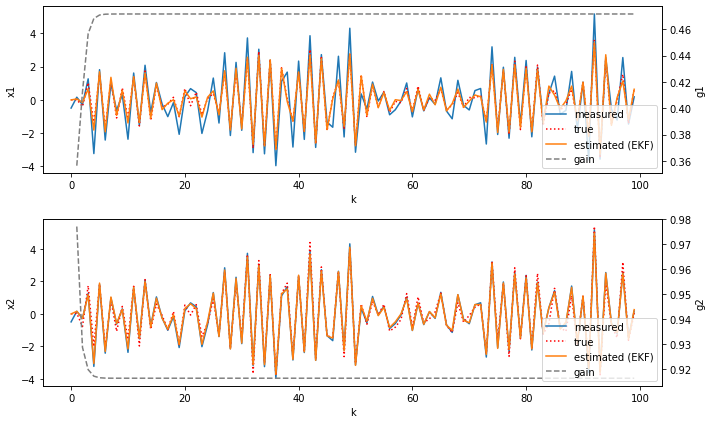
線形カルマンフィルタへの適用例

拡張カルマンフィルタは，当然，線形カルマンフィルタの問題に適用できる．
書籍の例を，上の関数でシミュレーションしてみる．

例えば，例題6.3はこんな感じ．

# --- パラメータ ---
A = np.array([
    [0, -0.7],
    [1, -1.5]
])
B = np.array([
    [0.5],
    [1]
])
C = np.array([
    [0],
    [1]
])

N, Q, R = 100, 1, 0.1

# --- 関数 ---
def f(x):
    return A @ x

def h(x):
    return C.T @ x

def dfdx(x):
    return A

def dhdx(x):
    return C.T

# --- 真値，　測定値 ---
v = np.random.normal(loc = 0.0, scale = np.sqrt(Q), size = N)
w = np.random.normal(loc = 0.0, scale = np.sqrt(R), size = N)

x = [np.array([[0], 
               [0]])]
y = [h(x[-1]) + w[0]]
for k in range(N - 1):
    x.append(f(x[-1]) + B * v[k + 1])
    y.append(h(x[-1]) + w[k + 1])
x = np.array(x)
y = np.array(y)

# --- EKF ---
gamma = 1
P_ekf = gamma * np.eye(2)
xhat_ekf, G_ekf = calc_timeseries_ekf(N, f, h, dfdx, B, dhdx, Q, R, y, x[0], P_ekf)

# --- プロット ---
fig_num = 2
fig = plt.figure(figsize = (10, 3 * fig_num), tight_layout = True)
axes = [fig.add_subplot(fig_num, 1, i + 1) for i in range(fig_num)]
for i in range(fig_num):
    ax = axes[i]
    ax2 = ax.twinx()
    ax.plot(y[:, 0, 0], label = 'measured', c = 'tab:blue')
    ax.plot(x[:, i], label = 'true', ls = 'dotted', c = 'red')
    ax.plot(xhat_ekf[:, i], label = 'estimated (EKF)', c = 'tab:orange')
    ax2.plot(G_ekf[:, i], label = 'gain', ls = 'dashed', c = 'tab:gray')
    ax.set_xlabel('k')
    ax.set_ylabel(f'x{i + 1}')
    ax2.set_ylabel(f'g{i + 1}')
    lines, labels = ax.get_legend_handles_labels()
    li2, la2 = ax2.get_legend_handles_labels()
    lines += li2
    labels += la2
    ax2.legend(lines, labels, loc = 'lower right')
plt.show()